library(Biostrings)     # version 2.70.3
library(rtracklayer)    # version 1.62.0
library(GenomicRanges)  # version 1.54.1
library(circlize)       # version 0.4.16
library(data.table)     # version 1.17.8
library(RColorBrewer)   # version 1.1-3
library(ggsci)          # version 4.0.0
library(scales) R scripts for: “Hybrid genome assemblies of R. sphaeroides DSM158 and its substrain H2”
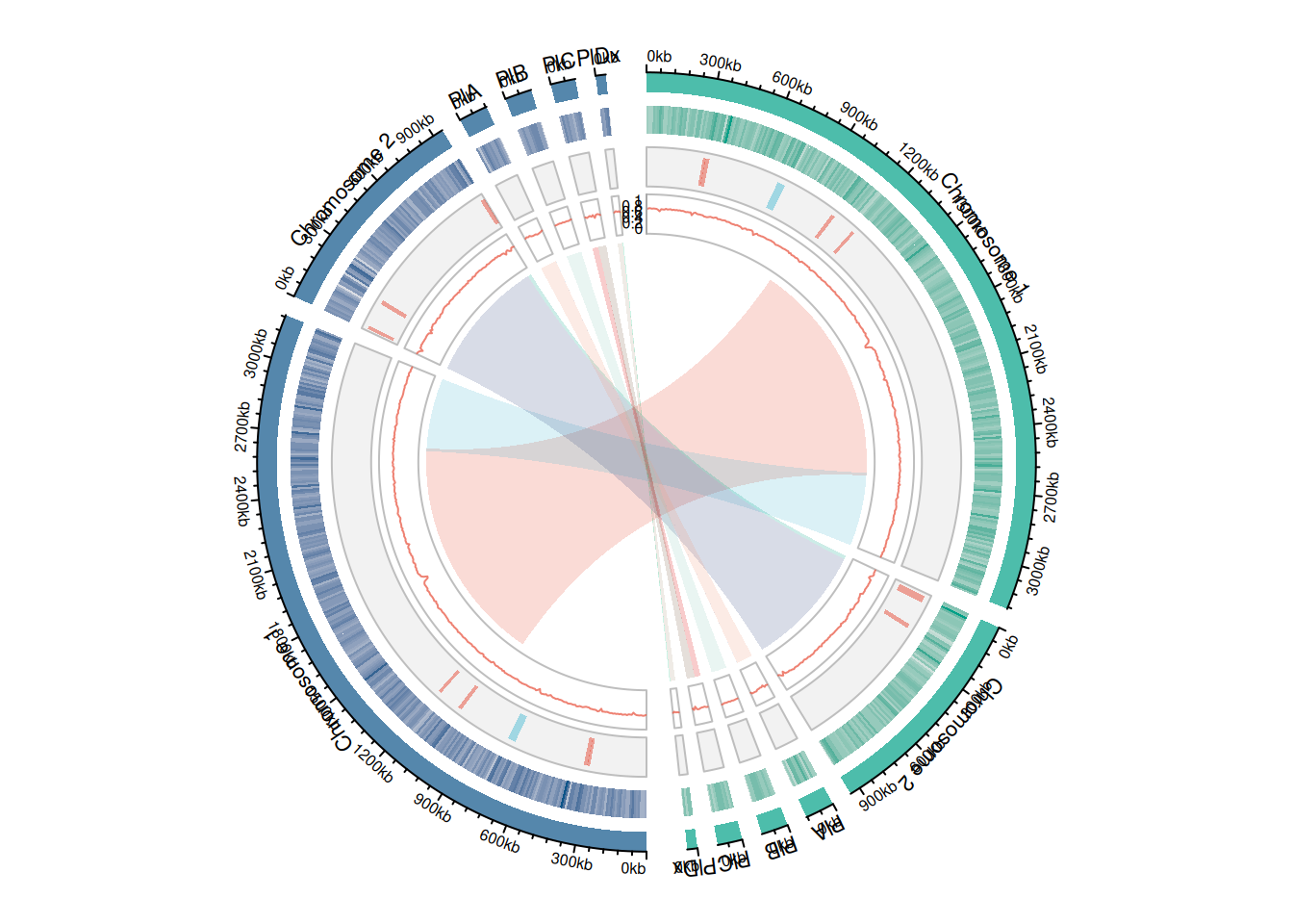
Circos plot of the assemblies using circlize
Loading the required packages
Import the genomes and the genome annotations
genomeA <- readDNAStringSet("/home/Drives/HDD03_06T_SDE/anna/SyntenyPlotDSMSubH2/DSM158/Cereibacter_sphaeroides_reoriented.fasta")
gffA <- import("/home/Drives/HDD03_06T_SDE/anna/SyntenyPlotDSMSubH2/DSM158/annot.gff")

genomeB <- readDNAStringSet("/home/Drives/HDD03_06T_SDE/anna/SyntenyPlotDSMSubH2/SubH2/GCF_049434525.1_MWCSPHH2ANNA_genomic.fasta")
gffB <- import("/home/Drives/HDD03_06T_SDE/anna/SyntenyPlotDSMSubH2/SubH2/genomic.gff")
Tidying the sequence names (remove file extension) and rename the chromosomes
#remove the file extensions (.fasta or .gff) from the sequence names
names(genomeA) <- sub(" .*", "", names(genomeA))
names(genomeB) <- sub(" .*", "", names(genomeB))
seqlevels(gffA) <- sub(" .*", "", seqlevels(gffA))
seqlevels(gffB) <- sub(" .*", "", seqlevels(gffB))

#Rename the chromosomes A_... or B_...
new_namesA <- paste0("A_", names(genomeA))
new_namesB <- paste0("B_", names(genomeB))

#Extract the lengths for each chromosome
chrom_lensA <- data.frame(chr=new_namesA, start=0, end=width(genomeA))
chrom_lensB <- data.frame(chr=new_namesB, start=0, end=width(genomeB))
chrom_lens <- rbind(chrom_lensA, chrom_lensB)

#Initialize the sectors for circlize
chrom_lens$chr <- as.character(chrom_lens$chr)
Create a sliding window (for the calculation of gene densities and GC content) of size 10,000 bp
win_size <- 10000
windowsA <- tileGenome(seqlengths(genomeA), tilewidth=win_size, cut.last.tile.in.chrom=TRUE)
windowsB <- tileGenome(seqlengths(genomeB), tilewidth=win_size, cut.last.tile.in.chrom=TRUE)
Calculate the gene densities
genesA <- gffA[gffA$type=="gene"]
gene_countsA <- countOverlaps(windowsA, genesA)
gendichteA <- data.frame(
  chr=factor(paste0("A_", seqnames(windowsA)), levels=new_namesA),
  start=start(windowsA), end=end(windowsA), value=gene_countsA
)

genesB <- gffB[gffB$type=="gene"]
gene_countsB <- countOverlaps(windowsB, genesB)
gendichteB <- data.frame(
  chr=factor(paste0("B_", seqnames(windowsB)), levels=new_namesB),
  start=start(windowsB), end=end(windowsB), value=gene_countsB
)
Calculate the GC content
calc_gc <- function(genome, windows, prefix) {
  vals <- numeric(length(windows))
  for (i in seq_along(windows)) {
    chr <- as.character(seqnames(windows[i]))
    seq <- subseq(genome[[chr]], start(windows[i]), end(windows[i]))
    vals[i] <- sum(letterFrequency(seq, c("G","C"), as.prob=TRUE))
  }
  data.frame(
    chr=factor(paste0(prefix, seqnames(windows)), levels=c(new_namesA,new_namesB)),
    start=start(windows), end=end(windows), value=vals
  )
}

gcA <- calc_gc(genomeA, windowsA, "A_")
gcB <- calc_gc(genomeB, windowsB, "B_")
Data for the phage sequences (PHASTER web-server)
repeatA <- data.frame(
  chr = c("1","1","1","1", "1", "2", "2", "2"),
  start = c(299942, 312405, 714792, 1045831, 1184739, 16443, 36955, 184600),
  end   = c(314808, 334525, 756993, 1067027, 1202250, 38142, 54813, 208162),
  type  = c("Incomplete","Incomplete","Questionable","Incomplete", "Incomplete","Incomplete", "Incomplete","Incomplete")
)
repeatB <- data.frame(
  chr = c("NZ_CP186561.1","NZ_CP186561.1","NZ_CP186561.1","NZ_CP186561.1", "NZ_CP186561.1", "NZ_CP186562.1", "NZ_CP186562.1", "NZ_CP186562.1"),
  start = c(299941, 312404, 714790, 1045832, 1184740, 9996, 157638, 920625),
  end   = c(314807, 333081, 756989, 1067028, 1202251, 27853, 181200, 944010),
  type  = c("Incomplete","Incomplete","Questionable","Incomplete", "Incomplete","Incomplete", "Incomplete","Incomplete")
)
repeatA$chr <- paste0("A_", repeatA$chr)
repeatB$chr <- paste0("B_", repeatB$chr)
repeat_df <- rbind(repeatA, repeatB)
Read the coordinates from a MUMMer coordinates file (for the synteny track)
read_mummer_coords <- function(file){
  raw <- readLines(file)
  header_line <- grep("\\[S1\\]", raw)
  data_lines <- raw[(header_line+2):length(raw)]
  data_clean <- gsub("\\|", "", data_lines)
  data_clean <- gsub("\\s+", " ", data_clean)
  coords <- read.table(text=data_clean, header=FALSE, stringsAsFactors=FALSE)
  if(ncol(coords)==8){
    colnames(coords) <- c("startA","endA","startB","endB","lenA","lenB","identity","chrA")
    coords$chrB <- coords$chrA
  } else if(ncol(coords)==11){
    colnames(coords) <- c("startA","endA","startB","endB",
                          "lenA","lenB","identity",
                          "lenRef","lenQry","chrA","chrB")
  } else if(ncol(coords)==13){
    colnames(coords) <- c("startA","endA","startB","endB",
                          "lenA","lenB","identity",
                          "lenRef","lenQry","covRef","covQry","chrA","chrB")
  } else {stop("Unbekanntes Format!")}
  coords
}

coords <- read_mummer_coords("/home/Drives/HDD03_06T_SDE/anna/SyntenyPlotDSMSubH2/MUMer/synteny.coords")
synteny <- data.frame(
  chrA = paste0("A_", coords$chrA),
  startA = coords$startA,
  endA = coords$endA,
  chrB = paste0("B_", coords$chrB),
  startB = coords$startB,
  endB = coords$endB
)
Color palette for the links (npg palette from the ggsci package) and for the other tracks
link_colors <- c(pal_npg("nrc", alpha = 0.2)(10),
                 alpha("#00d087B2",0.2),
                 alpha("#0c5f88b2",0.2)
                 )

colorA <- "#00a087B2"  # Green for genome A (DSM158)
colorB <- "#0c5488b2"  # Blue for genome B (SubH2)

# match genomes wth colors
chrom_colors <- ifelse(grepl("^A_", chrom_lens$chr), colorA, colorB)
Prepare the new chromosome names
# Chromosome-IDs in the plot
chrom_ids <- chrom_lens$chr

# New names (ordered)
new_labels <- c("Chromosome 1", "Chromosome 2", "PlA",
                "PlB", "PlC", "PlDx","Chromosome 1",
                "Chromosome 2", "PlA", "PlB", "PlC", "PlDx")

# Control if there are the same number og new labels and old labels
stopifnot(length(chrom_ids) == length(new_labels))

# Match new labels and old labels
names(new_labels) <- chrom_ids
Circos plot
circos.clear()
circos.par("start.degree"=90, gap.degree=c(rep(3,5),6,rep(3,5),6), cell.padding = c(0.02, 0, 0.02, 0), track.margin=c(0.01,0.01))

circos.initialize(factors=chrom_lens$chr,
                  xlim=cbind(chrom_lens$start, chrom_lens$end))

# Chromosomes at the outside
circos.trackPlotRegion(
  ylim=c(0,1),
  track.height=0.05,
  bg.border=NA,
  bg.col = chrom_colors,
  panel.fun=function(x,y){
    chr <- CELL_META$sector.index
    circos.text(
      CELL_META$xcenter,
      CELL_META$ycenter+ mm_y(4),
      col = "black",
      labels = new_labels[chr],   # Choosing name for each sector
      facing="inside",
      niceFacing=F,
      cex=0.7
    )
    circos.genomicAxis(h="top", labels.cex = 0.5)
  }
)
Note: 1 point is out of plotting region in sector 'A_1', track '1'.Note: 1 point is out of plotting region in sector 'A_2', track '1'.Note: 1 point is out of plotting region in sector 'A_3', track '1'.Note: 1 point is out of plotting region in sector 'A_4', track '1'.Note: 1 point is out of plotting region in sector 'A_5', track '1'.Note: 1 point is out of plotting region in sector 'A_6', track '1'.Note: 1 point is out of plotting region in sector 'B_NZ_CP186561.1',
track '1'.Note: 1 point is out of plotting region in sector 'B_NZ_CP186562.1',
track '1'.Note: 1 point is out of plotting region in sector 'B_NZ_CP186563.1',
track '1'.Note: 1 point is out of plotting region in sector 'B_NZ_CP186564.1',
track '1'.Note: 1 point is out of plotting region in sector 'B_NZ_CP186565.1',
track '1'.Note: 1 point is out of plotting region in sector 'B_NZ_CP186566.1',
track '1'.# Track 1: gene densities
maxA <- max(gendichteA$value)
maxB <- max(gendichteB$value)
col_funA <- colorRamp2(c(0, maxA), c("#eeeeee", "#00a087B2")) # grey → green
col_funB <- colorRamp2(c(0, maxB), c("#eeeeee", "#0c5488b2")) # grey → blue
gendichte_df <- rbind(gendichteA, gendichteB)
circos.track(ylim=c(0,1), track.height=0.1, bg.border=NA,
panel.fun=function(region,value,...){
chr <- CELL_META$sector.index
idx <- gendichte_df$chr == chr
for(i in which(idx)){
col_use <- ifelse(grepl("^A_", chr), col_funA(gendichte_df$value[i]), col_funB(gendichte_df$value[i]))
circos.rect(gendichte_df$start[i], 0,
gendichte_df$end[i], 1,
col=col_use, border=NA)
}
})
# Track 2: Phage sequences
repeat_types <- unique(repeat_df$type)
colors_repeats <- setNames(pal_npg("nrc", alpha = 0.7)(2)[1:length(repeat_types)], repeat_types)
circos.track(
ylim = c(0,1),
track.height = 0.1,
bg.border = "grey",
bg.col = "grey95",
panel.fun = function(region, value, ...) {
chr <- CELL_META$sector.index
idx <- repeat_df$chr == chr
if(any(idx)) {
ybottom <- CELL_META$ylim[1]
ytop <- CELL_META$ylim[2]
circos.rect(
xleft = repeat_df$start[idx],
ybottom= ybottom,
xright = repeat_df$end[idx],
ytop = ytop,
col = adjustcolor(colors_repeats[repeat_df$type[idx]], alpha.f=0.7),
border = NA
)
}
}
)
# Track 3: GC content
gc_df <- rbind(gcA,gcB)
circos.track(ylim=c(0,1), track.height=0.1, bg.border="grey", bg.col=NA,
panel.fun=function(region,value,...){
chr <- CELL_META$sector.index
idx <- gc_df$chr == chr
circos.lines((gc_df$start[idx]+gc_df$end[idx])/2, gc_df$value[idx],
col="#e64b35b2", lwd=1)
})
first_chr <- chrom_lens$chr[1]
circos.yaxis(side="left", sector.index=first_chr,
labels.cex=0.5, col="darkgrey", labels.col="black", tick.length=mm_y(2))
# Innermost track: synteny
for(i in 1:nrow(synteny)){
if(synteny$chrA[i] %in% chrom_lens$chr &&
synteny$chrB[i] %in% chrom_lens$chr){
circos.link(
sector.index1=synteny$chrA[i],
point1=c(synteny$startA[i], synteny$endA[i]),
sector.index2=synteny$chrB[i],
point2=c(synteny$startB[i], synteny$endB[i]),
col = link_colors[i],
border=NA
)
}}
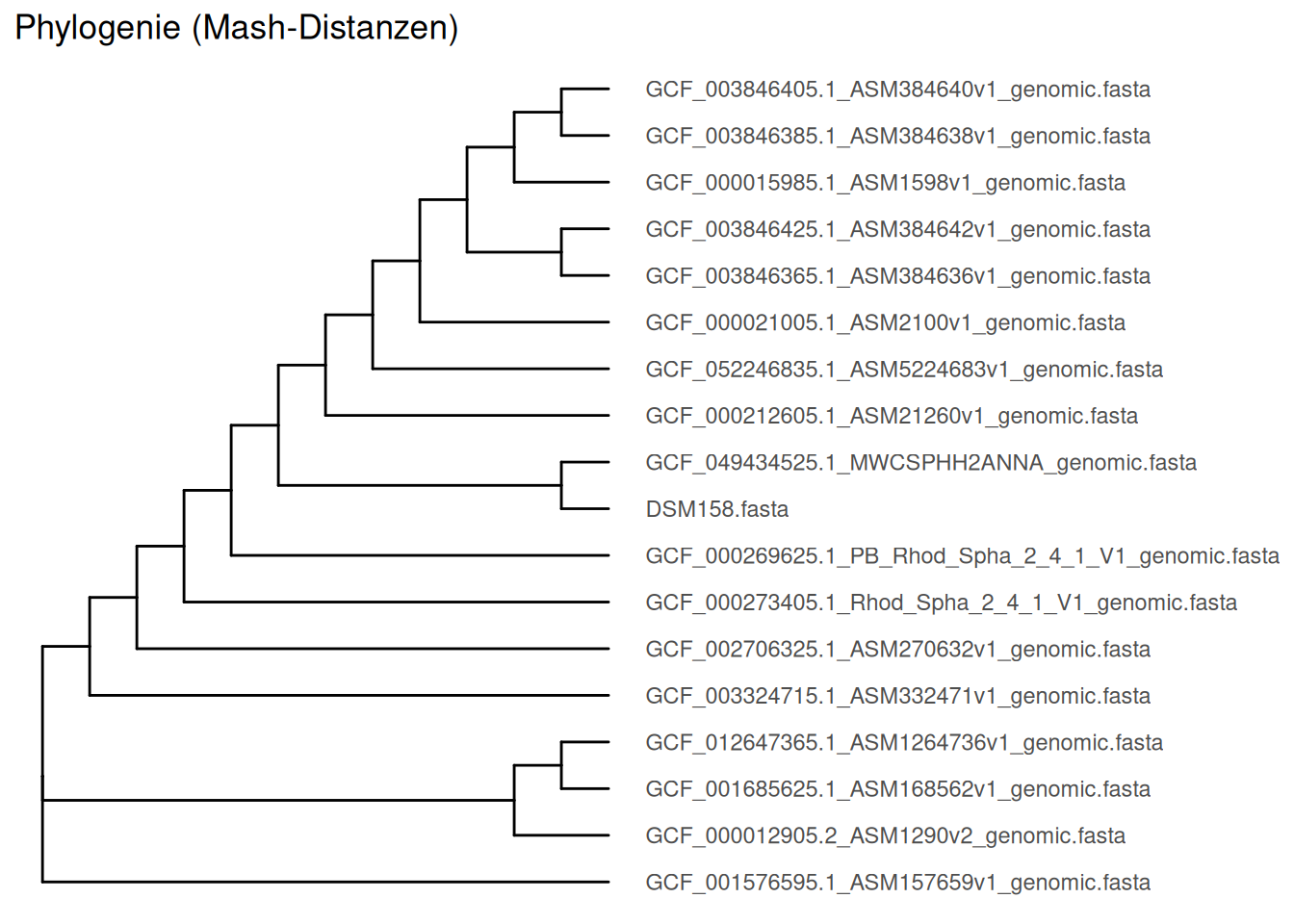
Synteny and phylogenetic tree of 18 complete R. sphaeroides genomes
Visualization of progressiveMauve Output
Loading required packages:
library(ggplot2)  # version 4.0.0
library(dplyr)    # version 1.1.4
library(stringr)  # version 1.5.1
library(scales)   # version 1.3.0
library(readxl)   # version 1.4.3
Function for parsing the progressiveMauve output
read_xmfa <- function(file) {
  lines <- readLines(file)
  cat("Number of read lines:", length(lines), "\n")

  blocks <- list()
  block_id <- 0
  current_block <- NULL

  for (line in lines) {
    # Skip comment lines
    if (startsWith(line, "#")) next

    # Block-deliminter
    if (trimws(line) == "=") {
      if (!is.null(current_block)) {
        blocks[[block_id]] <- current_block
        cat("Added Block", block_id, "with", nrow(current_block), "lines\n")
      }
      current_block <- NULL
      next
    }

    # Process header-lines
    if (startsWith(line, ">")) {
      cat("Process line:", line, "\n")
      # Example: >1:100-200 +
      pattern <- "^>\\s+([0-9]+):([0-9]+)-([0-9]+)\\s+([+-])\\s+(.*\\_*[0-9]+)\\.{1}.*"
      match <- regmatches(line, regexec(pattern, line))[[1]]

      if (length(match) == 6) {
        genome <- as.integer(match[2])
        start  <- as.integer(match[3])
        end    <- as.integer(match[4])
        strand <- match[5]
        genome_name <- match[6]

        if (is.null(current_block)) {
          block_id <- block_id + 1
          current_block <- data.frame(
            Genome = integer(),
            Start = integer(),
            End = integer(),
            Strand = character(),
            Block = integer(),
            Genome_Name = character(),
            stringsAsFactors = FALSE
          )
        }

        current_block <- rbind(current_block, data.frame(
          Genome = genome,
          Start = start,
          End = end,
          Strand = strand,
          Block = block_id,
          Genome_Name = genome_name,
          stringsAsFactors = FALSE
        ))
      } else {
        cat("No match for line:", line, "\n")
      }
    }
  }

  # Add last block, if available
  if (!is.null(current_block)) {
    blocks[[block_id]] <- current_block
    cat("Added last block", block_id, "with", nrow(current_block), "lines\n")
  }

  # Convert all blocks into one dataframe
  df <- do.call(rbind, blocks)
  cat("Final number of rows in the dataframe:", nrow(df), "\n")
  return(df)
}
Some important additional data
Location of the progressiveMauve output (
xmfa_file)Custom genome order, here as vector (
genome_order)An excel file listing all contig boundaries (
df)
xmfa_file <- "/home/Drives/HDD03_06T_SDE/anna/SyntenyPlotDSMSubH2/genomes/reoriented/C_sph_genomes.xmfa"

genome_order <- c("GCF_001576595", "GCF_000012905", "GCF_001685625",
                  "GCF_012647365", "GCF_003324715", "GCF_002706325",
                  "GCF_000273405", "GCF_000269625", "DSM158",
                  "GCF_049434525", "GCF_000212605", 'GCF_052246835',
                  "GCF_000021005", "GCF_003846365", "GCF_003846425",
                  "GCF_000015985", "GCF_003846385", "GCF_003846405")

df <- read_excel("/home/anna/R/Genome_Overview_Rsph.xlsx")
Reading the xmfa file
To simplify the visualization only blocks located in two or more assemblies are processed. Therefor we removed all unique blocks (xmfa_data_short).
xmfa_data <- read_xmfa(xmfa_file)

xmfa_data_short <- xmfa_data[(1:1683),]
To plot the different data together, we need to reorder our dataframes (df and xmfa_data_short) after the genome_order vector
df$Genome_Name <- factor(
  df$Genome_Name,
  levels = genome_order
)

xmfa_data_short$Genome_Name <- factor(
  xmfa_data_short$Genome_Name,
  levels = genome_order
)
Plotting the data with ggplot2
ggplot(xmfa_data_short,
       aes(y = Genome_Name)
  ) +
  geom_rect( #LCB from progressiveMauve
    aes(xmin = Start, xmax = End,
        ymin = as.numeric(Genome_Name) - 0.3,
        ymax = as.numeric(Genome_Name) + 0.3,
        fill = factor(Block))
  ) +
  geom_segment( #Contig boundaries
    data = df,
    aes(
      x = Contig_Boundaries_cum,
      xend = Contig_Boundaries_cum,
      y = as.numeric(Genome_Name) - 0.4,
      yend = as.numeric(Genome_Name) + 0.4
    ),
    color = "grey20",
    linetype = "dashed",
    linewidth = 0.3
  ) +
  scale_y_discrete(limits = genome_order) + # custom genome order
  guides(fill = "none")+ #remove legend
  theme_minimal()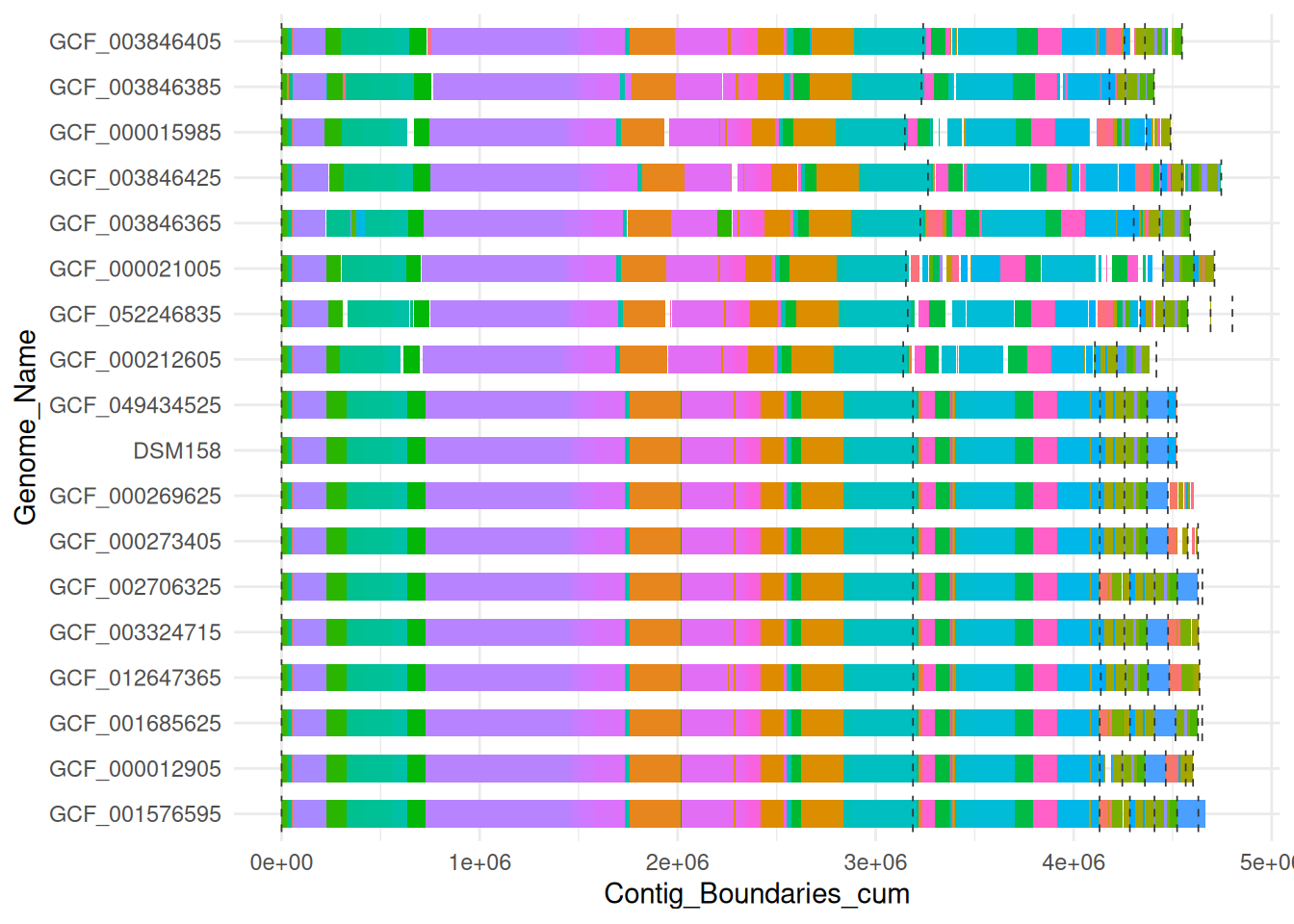
#Finetuning of the figure is made with inkscapeGenerating a phylogeny tree using a distance matrix from mash
Loading the required packages
library(ape) # version 5.7-1
Attaching package: 'ape'The following object is masked from 'package:dplyr':
whereThe following object is masked from 'package:circlize':
degreeThe following object is masked from 'package:Biostrings':
complementlibrary(tidyverse) # version 2.0.0── Attaching core tidyverse packages ──────────────────────── tidyverse 2.0.0 ──
✔ forcats 1.0.0 ✔ readr 2.1.5
✔ lubridate 1.9.3 ✔ tibble 3.2.1
✔ purrr 1.0.2 ✔ tidyr 1.3.1── Conflicts ────────────────────────────────────────── tidyverse_conflicts() ──
✖ lubridate::%within%() masks IRanges::%within%()
✖ dplyr::between() masks data.table::between()
✖ readr::col_factor() masks scales::col_factor()
✖ dplyr::collapse() masks Biostrings::collapse(), IRanges::collapse()
✖ dplyr::combine() masks BiocGenerics::combine()
✖ purrr::compact() masks XVector::compact()
✖ dplyr::desc() masks IRanges::desc()
✖ purrr::discard() masks scales::discard()
✖ tidyr::expand() masks S4Vectors::expand()
✖ dplyr::filter() masks stats::filter()
✖ dplyr::first() masks data.table::first(), S4Vectors::first()
✖ lubridate::hour() masks data.table::hour()
✖ lubridate::isoweek() masks data.table::isoweek()
✖ dplyr::lag() masks stats::lag()
✖ dplyr::last() masks data.table::last()
✖ lubridate::mday() masks data.table::mday()
✖ lubridate::minute() masks data.table::minute()
✖ lubridate::month() masks data.table::month()
✖ ggplot2::Position() masks BiocGenerics::Position(), base::Position()
✖ lubridate::quarter() masks data.table::quarter()
✖ purrr::reduce() masks GenomicRanges::reduce(), IRanges::reduce()
✖ dplyr::rename() masks S4Vectors::rename()
✖ lubridate::second() masks data.table::second(), S4Vectors::second()
✖ lubridate::second<-() masks S4Vectors::second<-()
✖ dplyr::slice() masks XVector::slice(), IRanges::slice()
✖ purrr::transpose() masks data.table::transpose()
✖ lubridate::wday() masks data.table::wday()
✖ lubridate::week() masks data.table::week()
✖ ape::where() masks dplyr::where()
✖ lubridate::yday() masks data.table::yday()
✖ lubridate::year() masks data.table::year()
ℹ Use the conflicted package (<http://conflicted.r-lib.org/>) to force all conflicts to become errorslibrary(reshape2) # version 1.4.4
Attaching package: 'reshape2'

The following object is masked from 'package:tidyr':

    smiths

The following objects are masked from 'package:data.table':

dcast, meltlibrary(ggplot2) # version 4.0.0
library(ggtree) # version 3.99.0ggtree v3.99.0 Learn more at https://yulab-smu.top/contribution-tree-data/
Please cite:
Shuangbin Xu, Lin Li, Xiao Luo, Meijun Chen, Wenli Tang, Li Zhan, Zehan
Dai, Tommy T. Lam, Yi Guan, Guangchuang Yu. Ggtree: A serialized data
object for visualization of a phylogenetic tree and annotation data.
iMeta 2022, 1(4):e56. doi:10.1002/imt2.56
Attaching package: 'ggtree'
The following object is masked from 'package:tidyr':
expand
The following object is masked from 'package:ape':
rotate
The following object is masked from 'package:Biostrings':
collapse
The following object is masked from 'package:IRanges':
collapse
The following object is masked from 'package:S4Vectors':
expandLoading the output from mash:
It should be a comma-separated file with the following columns:
Column 1: Name of the first genome
Column 2: Name of the second genome
Column 3: Distance between the genomes
Then we calculated the distance matrix
# Mash output: col1=genome1, col2=genome2, col3=distance
dist_tab <- read.table("/home/Drives/HDD03_06T_SDE/anna/SyntenyPlotDSMSubH2/mash/dist.tab",
                       header=FALSE,
                       stringsAsFactors = FALSE)

# Calculate distance matrix
dist_mat <- reshape2::acast(dist_tab, V1~V2, value.var="V3", fill=0)
dist_mat <- as.dist(dist_mat)
We used the distance matrix to calculate the neighbor-joining tree and plotted this tree using ggtree
# Neighbor-Joining tree calculation
tree <- nj(dist_mat)

#set global option to ignore negative edges
options(ignore.negative.edge=TRUE)
#plotting the tree using ggtree
 ggtree(tree) +
  geom_tiplab(align = T, as_ylab = T) +
  geom_hilight(node = c(3,4), color = "lightgreen")
Scale for y is already present.
Adding another scale for y, which will replace the existing scale.